Shiken: JALT Testing & Evaluation SIG Newsletter
Vol. 13 No. 2. May 2009. (p. 19 - 23) [ISSN 1881-5537]
PDF PDF Version

Statistics Corner
Questions and answers about language testing statistics:

Choosing the Right Number of Components
or Factors in PCA and EFA

Photo of JD Brown, c. 2000
James Dean Brown
University of Hawai'i at Manoa


* QUESTION: In Chapter 7 of the 2008 book on heritage language learning that you co-edited with Kimi Kondo-Brown, a study (Lee and Kim, 2008) compares the attitudes of 111 Korean heritage language learners. On page 167 of that book, a principal components analysis (with varimax rotation) describes the relation of examining 16 purported reasons for studying Korean with four broader factors. Several questions come to mind. What is a principal components analysis? How does principal components analysis differ from factor analysis? What guidelines do researchers need to bear in mind when selecting “factors”? And finally, what is a Varimax rotation and why is it applied?

* ANSWER: This inquiry has four sub-questions: (a) What are principal components analysis (PCA) and exploratory factor analysis (EFA), how are they different, and how do researchers decide which to use? (b) How do investigators determine the number of components or factors to include in the analysis? (c) What is rotation, what are the different types, and how do researchers decide which to use? And, (d) how are PCA and EFA used in language test and questionnaire development? I have addressed the first question (a) in the previous column (Brown, 2009, pp. 26-30). I’ll attend to the second one (b) here, and answer the other two in subsequent columns.

Choosing the Number of Components or Factors to Include in a PCA or EFA

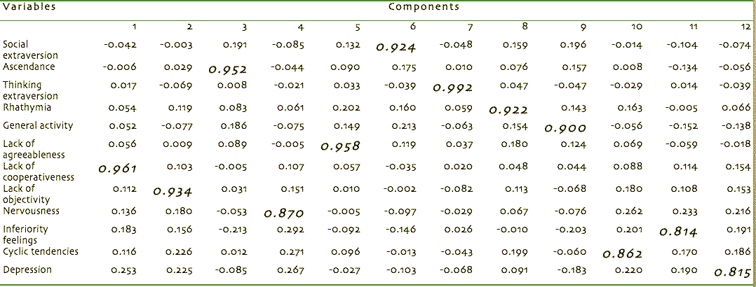
So, how do researchers decide on the number of components or factors to include in a PCA or EFA? If the researcher erroneously includes the same number of PCA components as there are variables (say 12 components in the 12-variable Y/GPI Brazilian university student example used in the previous Statistics Corner column), each factor will represent one variable as shown in Table 1. Such situations, where only one variable loads heavily in each column indicates that the factor scores for each factor essentially represent a single variable; the researcher already knew about the single variable, so such single loading “components” or “factors” do not represent any underlying combinations of variables that provide new or interesting information (see the discussion of trivial factors below).

Table 1. PCA Results for the 12 Y/GPI Scales Administered in Brazil with 12 Components Based on 12 Variables
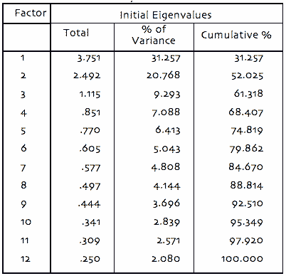
Table 1

* What researchers need instead is some way to determine a smaller number of factors or components (hereafter referred to collectively as factors) that account for large amounts of the overall variance without creating any bloated specifics. To that end, a number of “stopping rules” have been proposed to determine when the researcher should stop adding factors (see Bryant and Yarnold, 1995, pp. 102-104; Gorsuch, 1983, pp. 164-174). How does a research know how many factors to use? When should the researcher stop? There are various statistical tests to determine the optimum number of variables (Gorsuch, 1983, p. 143-164), but more commonly these non-statistical strategies are used:
"a number of 'stopping rules' have been proposed to determine when the researcher should stop adding factors."
  1. Kaiser's stopping rule
  2. Scree test
  3. Number of non-trivial factors
  4. A priori criterion
  5. Percent of cumulative variance

[ p. 19 ]

Each of these topics will now be explained and exemplified in turn.

Examples Illustrating the Five Stopping Rules

I will base this discussion on the same example used in the previous column. Recall that the data were based on the 12 subtests of the Y/G Personality Inventory (Y/GPI) (Guilford and Yatabe, 1957) which were: social extraversion, ascendance, thinking extraversion, rhathymia, general activity, lack of agreeableness, lack of cooperativeness, lack of objectivity, nervousness, inferiority feelings, cyclic tendencies, and depression. The data were based on an English language version of the Y/GPI administered to 259 students at two universities in Brazil for comparative purposes. The descriptive results for these data were shown in Table 2 of the previous column.
Because ample theory and research indicate that the first six subtests are extraversion scales and the remaining six pertain to neuroticism (for more on the Y/GPI, see Guilford and Yatabe, 1957; Robson, 1994; Brown, Robson, and Rosenkjar, 2001), it would probably make sense to perform the EFA instead of PCA (as discussed in the last Statistics Corner column). Let’s consider each of the five ways of deciding on the appropriate number of factors when they are applied to the example data. (1) Kaiser's stopping rule
Kaiser’s stopping rule states that only the number of factors with eigenvalues over 1.00 should be considered in the analysis. The initial analysis of the example data indicated that three factors had an eigenvalue of 1.00 or higher (see Table 2 which is taken directly from the initial analysis SPSS output). Notice in Table 2 that the Factors 1, 2, and 3 (labeled in the first column) have eigenvalues of 3.751, 2.492, and 1.115, respectively. Thus all three are above Kaiser’s cut-point of 1.00. Factors 4 to 12 are below that cut-point with values of .851 down to .250.

Table 2. Initial EFA for the 12 Y/GPI Scales Administered in Brazil
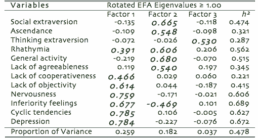
Table 2
Table 3. EFA (with Varimax Rotation) Loadings for the 12 Y/GPI Scales Administered in Brazil
Table 3

* Now consider the results shown in Table 3 for a three-factor EFA of the example data (with varimax rotation). Notice that the first column contains labels for the 12 scales. Then the next four columns show the results for the EFA including loadings, communalities (on the right), and proportions of variance (across the bottom). Factor 1 appears to have fairly strong loadings from the six neuroticism scales as expected. Factor 2 also has fairly high loadings from the first, second, fourth, fifth, and sixth extraversion scales. Notice that Rhathymia loads on both factors (such variables are referred to as complex, in this case, Rhathymia has a poor positive correlation with Factor 1 and a good positive correlation with Factor 2). Inferiority feelings also load on both factors (this variable is also complex, but in this case, it has a very good positive correlation with Factor 1 and a fair negative one with Factor 2). Also, surprisingly, the third extraversion scale (Thinking extraversion) does not load on Factor 1 or 2. Thus this variable does not seem to fit the theory developed in previous research. This result does not mean that the theory was wrong for the types of respondents that participated in the previous research. It does mean, however, that Thinking extraversion does not load on either Factor 1 or 2 for the types of Brazilian university students included in the data analyzed here. Indeed, Thinking extraversion has only one loading worth noting at 0.530, and that loading is just sitting there by itself and not forming a factor that is useful in any way. We will consider this situation further in the ensuing discussion.

[ p. 20 ]

(2) Scree test

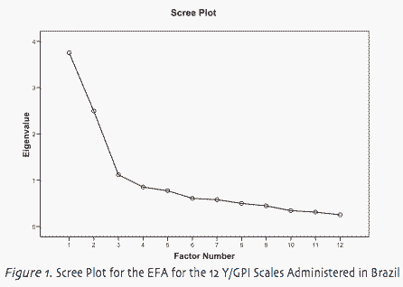
Another strategy for examining the eigenvalues is called the scree test. This strategy involves creating a graphic visualization of the relationship between eigenvalues and number of factors as shown in Figure 1.
Figure 1. Scree Plot for the EFA for the 12 Y/GPI Scales Administered in Brazil.
Table 4. EFA (with Varimax Rotation) Loadings for 2
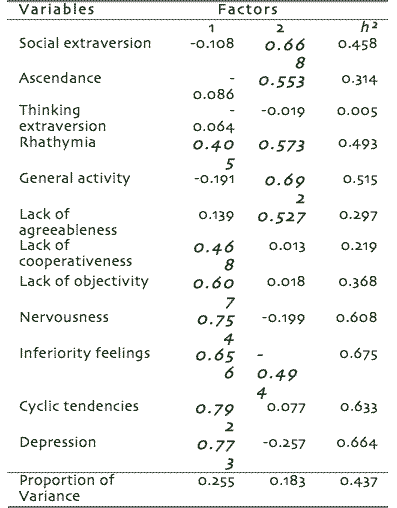
Table 4

* The scree plot is obviously a graph of the relationship between the relative magnitude of the eigenvalues and the number of factors. The researcher examines the scree plot and decides where the line stops descending precipitously and levels out (for more on scree plot interpretation, see Bryant and Yarnold, 1995, pp. 103-104).
In the case shown in Figure 1, that would appear to happen at three factors. The researcher then ignores all of the points along the level part of the line including the transition point, and counts the points along the precipitously dropping part of the line. Thus this particular scree plot indicates that a two-factor solution would be appropriate.
Table 4 presents just such a two-factor analysis—one in which all variables either load clearly on Factor 1 or 2 (or are complex, as explained above, in the case of Rhathymia and Inferiority feelings) except for Thinking extraversion, which loads on neither factor.

(3) Number of non-trivial factors.

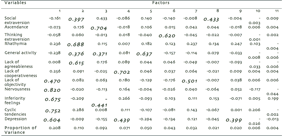
Trivial factors are usually defined as those that do not have two or three variables loading above the cut-point (often .30) on them. Table 5 shows the loadings from an EFA (with Varimax Rotation) for an 11-factor solution using the example data. Notice in Table 5 that only three factors can be said to have three or more loadings above the cut-point of .30. Factors 5 through 9 are clearly examples of single loading factors, and factors 10 and 11 have no loadings worth considering, while Factor 4 only has two variables loading above the cut-point of .30. All of this would seem to argue for either a three or four-factor solution.


1 Why is it called a scree test? Take a look at Figure 1 and try to visualize rocks and debris at the bottom of a cliff. See it? That stuff at the bottom of the cliff is called a scree in geology.
2 Note that Tabachnick and Fidell (2007, p. 646) suggest a cut-point of .32 and above "...then there is 10% or more overlap in variance among factors."

[ p. 21 ]


Table 5. EFA (with Varimax Rotation) Loadings for 11 Factors Using the 12 Y/GPI Scales Administered in Brazil
Table 4


However, there is the possibility that some factors may be trivial. In interpreting trivial and non-trivial factors, it is worth considering that triviality is a matter of degrees. According to Comrey and Lee (1992), loadings of .71 or higher can be considered “excellent”, .63 is “very good”, .55 is “good”, .45 is “fair”, and .32 is “poor”. So what magnitude is trivial? Clearly, higher loadings indicate variables that are more highly related to whatever the underlying factor is. Hence, variables with high loadings can be considered purer measures of the underlying factors. This means that two, three, or more loadings higher than .71 are clearly less trivial than say two loadings of .30 or .40.
In Table 5, based on the number of loadings and their absolute magnitude, it could be argued that Factors 1 and 2 are less trivial than say Factors 3 and 4. The problem is that triviality may be in the eye of the beholder.

(4) A priori criterion

If the researcher is replicating previous research wherein a specific number of factors were found, it would make sense to set that same number of factors in the replication research. Similarly, if a researcher has created a set of test or questionnaire items to contain a specific number of subtests or scales, it would make sense to set that same number of factors in the factor analysis of those items. These are known as a priori criteria for determining the number of factors. For example, in previous research on the Y/GPI, the 12 subscales were shown to fall into two general categories: extroversion and neuroticism. Thus, a two-factor solution for the example data (as shown in Table 4) would make theoretical sense based on a priori criteria drawn from previous research.

(5) Percent of cumulative variance

An approach that is closely related to Kaiser’s stopping rule and the scree plot is the percent of cumulative variance. However, percents of cumulative variance are harder to interpret than the other two. Clearly, in the example study, a 12 variable solution in a PCA would account for 100% of the variance, but as shown in Table 1, that would tell the researcher nothing. So some smaller number of factors should be sought. Looking down the far right column in Table 2 reveals the percentages of cumulative variance for various numbers of factors in that analysis. The addition of each factor adds some new variance to the cumulative variance. So where should the researcher stop? It is impossible to say.
As a result interpreting the percentages of cumulative variance is more a matter of keeping an eye on the amount of cumulative variance being accounted for by various other stopping rules. Close examination of the far right column in Table 2 indicates that 61.318% of the variance is accounted for if the three-factor solution (based on Kaiser’s stopping rule) is used, but, if the two-factor solution is adopted (based on the scree test), only 52.025% of the variance is accounted for.

Conclusion


3 Asking for 12 factors in an EFA with varimax rotation, SPSS warns: "You cannot request as many factors as variables with any extraction method except PC. The number of factors will be reduced by one."

[ p. 22 ]

"But which method is correct? I guess the safest answer is that no method is correct. Instead, some combination of the five sets of issues must be included in making the decision and explaining it to the readers of the resulting research report."
Clearly, there are a number of different ways to look at the issue of deciding how many components or factors to include in a PCA or EFA. I discussed Kaiser’s stopping rule, the scree test, the number of non-trivial factors, a priori criterion, and the percent of cumulative variance as different ways to make such decisions. Each of these methods indicated that there should be three or two factors. But which method is correct? I guess the safest answer is that no method is correct. Instead, some combination of the five sets of issues must be included in making the decision and explaining it to the readers of the resulting research report. The trick is to make the strongest possible set of arguments for why a particular number of factors were selected in a particular analysis. If an a priori criterion argument can be included that may prove the most convincing and useful, but the point is that the argument for the number of components or factors should be based on a combination of information from the five viewpoints explained here.
In the case of the example data used here, there was indeed a theory-based a priori criterion of two factors. In addition, the scree plot indicted that a two-factor solution was appropriate, and the percent of variance accounted for by a two-factor solution is about 44% (see bottom right corner of Table 4). Finally, three-factor solutions tended to produce a trivial third factor, while two-factor solutions clearly produced two non-trivial factors. All in all, I am most comfortable with a interpreting the two-factor solution based on all of these considerations.
Two things should be clear in this discussion of how researchers decide on the number of factors to include in a PCA or EFA. First, the decision must be based on the preponderance of evidence from all five perspectives on the issue. Second, this is not a clear-cut decision based on a set of yes/no questions; there is an art to deciding on and explaining why you decided on a specific number of components or factors. And, third, the abilities needed for making such decisions and explaining them to readers improve over time (though they will never be perfect) so don’t be afraid to critically read the explanations provided by researchers in second language studies, and indeed if you have testing, questionnaire, or other appropriate data of your own, don’t hesitate to dive in and see what you find with a PCA or EFA.

References

Brown, J. D. (2009). Statistics Corner. Questions and answers about language testing statistics: Principal components analysis and exploratory factor analysis: Definitions, differences, and choices. Shiken: JALT Testing & Evaluation SIG Newsletter, 13 (1) 26-30. Retrieved March 30, 2009 from http://jalt.org/test/bro_29.htm

Brown, J. D., Robson, G., & Rosenkjar, P. (2001). Personality, motivation, anxiety, strategies, and language proficiency of Japanese students. In Z. Dörnyei & R. Schmidt (Eds.), Motivation and second language acquisition (pp. 361-398). Honolulu, HI: Second Language Teaching & Curriculum Center, University of Hawai‘i Press.

Bryant, F. B., & Yarnold, P. R. (1995). Principal-components analysis and confirmatory factor analysis. In L. G. Grimm & P. R. Yarnold (Eds.), Reading and understanding multivariate statistics. Washington, DC: American Psychological Association.

Comrey, A. L., & Lee, H. B. (1992). A first course in factor analysis (2nd ed.). Hillsdale, NJ: Lawrence Erlbaum Associates.

Gorsuch, R. L. (1983). Factor analysis (2nd ed.). Hillsdale, NJ: Lawrence Erlbaum Associates.

Guilford, J. P., & Yatabe, T. (1957). Yatabe Guilford personality inventory. Osaka: Institute for Psychological Testing.

Kim, J. O., & Mueller, C. W. (1978). Introduction to factor analysis: What it is and how to do it. Beverly Hills, CA: Sage.

Lee, J. S., & H. Y. (2008). In K. Kondo-Brown & J. D. Brown (Eds.), Teaching Chinese, Japanese, and Korean heritage language students. New York: Lawrence Erlbaum Associates.

Robson, G. (1994). Relationships between personality, anxiety, proficiency, and participation. Unpublished doctoral dissertation, Temple University Japan, Tokyo, Japan.

Tabachnick, B. G., & Fidell, L. S. (2007). Using multivariate statistics (5th ed.). Upper Saddle River, NJ: Pearson Allyn & Bacon.


Where to Submit Questions:
Please submit questions for this column to the following address:
JD Brown
Department of Second Language Studies
University of Hawai'i at Manoa
1890 East-West Road
Honolulu, HI 96822 USA


NEWSLETTER: Topic IndexAuthor IndexTitle IndexDate Index
TEVAL SIG: Main Page Background Links Network Join

STATISTICS CORNER ARTICLES:
#1   #2   #3   #4   #5   #6   #7   #8   #9   #10   #11   #12   #13   #14   #15   #16   #17   #18   #19   #20   #21   #22   #23   #24   #25   #26   #27   #28   #29   #30   #31   #32   #33   #34  
last Main Page next
HTML: http://jalt.org/test/bro_30.htm   /   PDF: http://jalt.org/test/PDF/Brown30.pdf

[ p. 23 ]