Questions and answers about language testing statistics: Sample size and power

Shiken: JALT Testing & Evaluation SIG Newsletter
Vol. 11 No. 1. Mar. 2007. (p. 31 - 35) [ISSN 1881-5537]

Statistics Corner
Questions and answers about language testing statistics:

Sample size and power

James Dean Brown
University of Hawai'i at Manoa

QUESTION: One topic I think many people would be interested in is something about sampling sizes and calculating sampling errors. It seems many teachers just randomly select a number between 20 – 50 when determining the size of their samples without knowing why (or how) a sample size for a survey should estimate – or how to calculate the error of measurement that is probably due to sampling error. Since most of the research studies language teachers in Japan conduct involve small samples, some information about calculating sampling errors is probably needed.

ANSWER: As I pointed out in my last column (Brown, 2006), you seem to be asking several questions simultaneously: one about sampling and generalizability, and at least two others about sample size and statistical precision and power. I addressed the first question (sampling and generalizability) in my last column. In this one, I will discuss sample size as it relates to power. However, I will kick the can of precision a bit further down the road, by discussing it in the next column.

Null Hypotheses

To lay some groundwork, I must first define the notion of the null hypothesis (H₀), which is "the hypothesis that the phenomenon to be demonstrated is in fact absent" (Fisher, 1971, p. 13). For example, it is the hypothesis that there is no correlation (r = 0), or that there is no difference between the means (M₁ = M₂) in a t-test, or that there is no difference between the observed and expected frequencies (∫_o = ∫_e) in a t-test. The null hypothesis is important because it is what L2 researchers are most often testing in their studies. If they can reject the null hypothesis at a certain alpha level (e.g., p < .05), then they can accept as probable whatever alternative hypothesis makes sense, for example, that the correlation is a non-chance occurrence (e.g., r < 0 at p < .05), or that the first mean is greater than the second mean for reasons other than chance (e.g., M₁ < M₂ at p < .05) in a t-test, or that the observed frequency is greater than the expected frequency due to factors other than chance (e.g., ∫_o < ∫_e at p < .05). Once again, focusing on rejecting the null hypothesis and declaring a "significant" (at p < .05) correlation, mean difference, or difference between observed and expected frequencies is how L2 researchers typically proceed.

Type I vs. Type II Errors

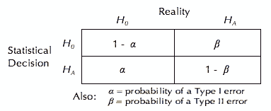
Most often, the probability statements in the above examples are taken to indicate the probability that the researcher will accept the alternative hypothesis when in reality the null hypothesis is true (see α in lower-left corner of Figure 1). That seems to be the primary concern of most researchers in L2 studies. However, there is another way to look at these issues that involves what are called Type I and Type II errors. From this perspective, α is the probability of making a Type I error (accepting the alternative hypothesis when in reality the null hypothesis is true), and β is the probability of making a Type II error (accepting the null hypothesis when in reality the alternative hypothesis is true). By extension, 1 - α is the probability of not making a Type I error, and 1 - β is the probability of not making a Type II error.

[ p. 31 ]

Figure 1. Four ways of looking at the probabilities in statistical tests

As I mentioned above, the primary concern of most researchers in L2 studies (indeed in most social sciences) is to guard against Type I errors, errors that would lead to interpreting observed correlations, mean differences, frequency differences, etc. as non-chance (or probably real) when they are in reality due to chance fluctuations. However, researchers in our field seldom think about Type II errors and their importance. Recall that Type II errors are those that might lead us to accept that a set of results is null (i.e., there is nothing in the data but chance fluctuations) when in reality the alternative hypothesis is true. L2 researchers may be making Type II errors every time they accept the null hypothesis because they are so tenaciously focused on Type I errors (α) while completely ignoring Type II errors (β). What is the solution to this problem? We should calculate β every time we do an analysis. But this is difficult, right? No, with programs like SPSS, we can easily calculate power (1 - β) for many analyses (see explanation below). Then, once we know 1 - β, we can also calculate β by subtracting the power statistic from 1. Thus results like those shown in Figure 2 can easily be obtained for many analyses.

Figure 2. Four probabilities worth thinking about in a hypothetical study

What is Power?

In the simplest terms, the power of a statistical test is "the probability that it [i.e., the statistical test] will lead to the rejection of the null hypothesis, i.e., the probability that it will result in the conclusion that the phenomenon exists" (Cohen, 1988, p. 4). Thus power is the 1 - βin Figures 1 and 2, which turned out to be .82. But is that high enough? How much power is enough? Cohen (1988, p. 56, and elsewhere) discussed this issue and proposed that, "…when the investigator has no other basis for setting the desired power value, the value .80 be used. This means that β is set at .20." Thus in the same sense that researchers conventionally set the cut-point for α at .05 or .01, the cut-point for β can reasonably be set at less than .20 (or greater than .80 for power). As a result, we can say that the power of .82 shown in Figure 2 indicates that the study had sufficient statistical power for the researcher to accept the alternative hypothesis with a fair amount of confidence. By extension, we can say that power of .82 indicates that β = .18 (1.00 - β = 1.00 - .82 = .18) and that the probability of accepting the null hypothesis when in reality the alternative hypothesis is true is only .18.

[ p. 32 ]

What Sorts of Errors Do L2 Researchers Make by Ignoring Power

The two most common Type II errors that L2 researchers make are those that have to do with (a) establishing the equivalence of groups at the beginning of a study and (b) not knowing what to do with null results when they arise in the main analyses of a study. I will use examples from papers published by Mason (2004) and Kondo-Brown (2001) because they illustrate the issues involved and because they are both Japan-related studies.

Errors related to the equivalence of groups at the beginning of a study. Mason (2004, p. 8) implies that the groups in her study were the same at the beginning of her study when she writes, "A one-way ANOVA showed that there was no significant difference among the groups on the pretest,F(2, 93) = 1.514, p = .225." The problem of course is that a non-significant difference like this one indicates that α (or the probability of accepting the alterative hypothesis when in reality the null hypothesis is true) is .225. It does not indicate β (the probability of accepting the null hypothesis when in reality the alternative hypothesis is true). The alternative hypothesis that the means are different could still be true in Mason's study, but remain undetected because of weak research design (too small a sample size, low reliability in the measurements, etc.). This is a common Type II error made in L2 research. She is accepting the null hypothesis when in reality the alternative hypothesis could be true. If she had calculated 1 - β (power) and it had turned out to be .80 or higher (with a corresponding β of .20 or lower), she would then have been in a position to make the interpretation that she did. But she didn't do that and so she will never know what the most probable cause is of the null result. Many L2 researchers have made this mistake. That needs to change.

Errors resulting from not knowing what to do with null results. As good researchers often do in our field nowadays, Mason (2004, p. 8) set her alpha level low at .01 in her main analysis because she recognized a potential for Type I errors: "The alpha level was set at .01, as multiple ANOVAs were used for the analyses." However, she did not recognize the potential threat from Type II errors in the same analysis, when she wrote: "All three groups in this study improved significantly, but there were no significant differences among the groups in gains. The group that wrote summaries in Japanese, their first language, was the most efficient, making the greatest gains in terms of points gained for the time devoted to English" (Mason, 2003, p. 15). Mason seems to be having trouble with the fact that she did not find statistically significant differences in her study between the groups. In effect, she chooses to accept the null between-groups results without justification. She then ignores the null results and proceeds to interpret the analysis in terms of efficiency.
If, instead, she had calculated power (1 - β), and it had turned out to be .80 or higher (with a corresponding β of .20 or lower), she would have had to acknowledge that her study had sufficient power to reject the null hypothesis, but had not done so, and that her observed differences could only be interpreted as chance fluctuations. If, on the other hand, the power had turned out to be .79 or lower, she could have discussed the design issues that might have caused the lack of power to detect significant differences. Either way her interpretation would have been clearer and more accurate than falling back on interpreting the lack of a statistically significant difference in terms of efficiency (after discovering that those null differences may have simply resulted from chance fluctuations).
Another example from Japan shows how knowing what to do with null results (i.e., knowing how power statistics can be effectively used to understand null results) can help a researcher grasp the meaning of the results of her statistical tests. Kondo-Brown (2001, p. 101) clearly did use power statistics and did so successfully in my view¹ when she wrote the following:

In fact, in a follow-up power analysis on the production tests, the observed power (1 - _), which is the probability of correctly rejecting the null hypothesis (Tabachnick & Fidell, 1996: 36-37), was 0.50 for the immediate posttest and 0.11 for the delayed posttest, both of which were fairly low (for more information about power analysis, see Cohen, 1988: Lipsey, 1990). This suggests that the design (i.e., n-size, distributions, and treatment magnitude) may not have been strong enough to detect significant differences.

¹ In the interest of full disclosure, I must confess that this top-notch researcher is in fact my wife, so I may be a bit biased in my assessment of her phenomenal abilities. That does not change the value of this example.

[ p. 33 ]

The bottom line with regard to power analysis is that there is much to be gained in our understanding of the statistical results of our studies if only we will ask our statistical programs to calculate power.

How Can We Calculate Power?

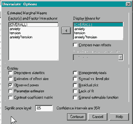
In many SPSS analyses, we can calculate power by asking for it as an option. For example, Figure 3 shows the Options window available in the GLM analyses for univariate ANOVA (in this case a 2 x 2 two-way ANOVA with anxiety and tension as the independent variables and trial 3 as the dependent variable using the Anxiety 2.sav example file that comes with SPSS v. 14). Notice that getting the power statistics was no more difficult than checking a box (see the results in Table 1 below).

Figure 3. Example of asking for power analysis in the options window in SPSS

Notice in Table 1 that the p values (0.90, 0.55, & 0.10) indicate that there were no significant differences (i.e., no p values below .05) for Anxiety, Tension, or their interaction, but also that there was not sufficient power to detect such effects (i.e., the power statistics of 0.05, 0.09, & 0.37 were not above .80 in any case). All of this leads to the quite reasonable conclusion that the study lacked sufficient power to detect any significant effects even if they exist in reality, in this case, it is probably because the sample size was a very small (n = 12) in a relatively complex 2 x 2 two-way ANOVA design.

Table 1. Results of the Analysis Shown in Figure 3

Conclusion

Clearly, L2 researchers would benefit from considering both Type I and Type II errors. Naturally, this will necessitate discussing not only α but also β and 1- β (power) in our studies so we can correctly accept the null hypotheses or alternative hypothesis in our various statistical tests. Equally important, power statistics can help us to better understand Type II threats in our studies, in particular, the degree to which the sample size, reliability of measurement, strength of treatment, etc. provide adequate power for finding a statistically significant result if in fact it exists. When you are doing your statistics, why not click on that observed power box while you are at it?

[ p. 34 ]

In a more direct answer to the original question, if the power of a statistical test is sufficient (i.e., is .80 or higher), the sample size is probably sufficient for the common research purposes discussed here. If the power statistic is not larger enough (i.e., is .79 or lower), the researcher might want to consider increasing the sample size and thereby just possibly raise the power of the study. Indeed, it is even possible to use the power statistic to estimate how much larger the sample should be. For an example of this use of power, see Gorsuch (1999, pp. 189-196). [For more on this and related topics, see Cohen, 1988; Kline, 2005; Kraemer & Thiemann, 1987; Lipsey, 1990; Murphy & Myors, 2004; Rosenthal, Rosnow, & Rubin, 2000; and Thompson, 2006.]

References

Brown, J. D. (2006). Statistics Corner. Questions and answers about language testing statistics: Generalizability from second language research samples. Shiken: JALT Testing & Evaluation SIG Newsletter, 10 (2), 24-27. Also retrieved from the World Wide Web at http://jalt.org/test/bro_24.htm

Cohen, J. (1988). Statistical power analysis for the behavioral sciences (2nd ed.). Hillsdale, NJ: Lawrence Erlbaum Associates.

Fisher, R. A. (1971). The design of experiments (8th ed.). New York: Hafner. Reproduced in J. H. Bennett (Ed.) (1995), Statistical methods, experimental design, and scientific inference. Oxford: Oxford University.

Kline, R. B. (2005). Beyond significance testing: Reforming data analysis methods in behavioral research. Washington, DC: American Psychological Association.

Kondo-Brown, K. (2001). Effects of three types of practice in teaching Japanese verbs of giving and receiving. Acquisition of Japanese as a Second Language, 4, 82-115.

Kraemer, H. C., & Thiemann, S. (1987). How many subjects? Statistical power analysis in research. Newbury Park, CA: Sage.

Lipsey, M. W. (1990). Design sensitivity: Statistical power for experimental research. Newbury Park, CA: Sage.

Mason, B. (2003). A study of extensive reading and the development of grammatical accuracy by Japanese university students learning English. Unpublished doctoral dissertation, Temple University, Philadelphia, PA.

Mason, B. (2004) The effect of adding supplementary writing to an extensive reading program. The International Journal of Foreign Language Teaching, 1 (1), 2-16. Also retrieved from the World Wide Web at http://www.tprstories.com/ijflt/IJFLTWinter041.pdf

Murphy, K. R., & Myors, B. (2004). Statistical power analysis: A simple and general model for traditional hypothesis tests (2nd ed.). Hillsdale, NJ: Lawrence Erlbaum Associates.

Rosenthal, R., Rosnow, R. L., & Rubin, D. B. (2000). Contrasts and effect sizes in behavioral research: A correlational approach. Cambridge: Cambridge University.

Tabachnick, B. G., & Fidell, L. S. (1996). Using Multivariate Statistics (3rd ed.). New York: HarperCollins College.

Tabachnick, B. G., & Fidell, L. S. (2001). Using Multivariate Statistics (5th ed.). Upper Saddle River, NJ: Pearson Allyn & Bacon.

Thompson, B. (2006). Foundations of behavioral statistics: An insight-based approach. New York: Guilford.

Where to Submit Questions:

Please submit questions for this column to the following address:

JD Brown
Department of Second Language Studies
University of Hawai'i at Manoa
1890 East-West Road
Honolulu, HI 96822 USA

NEWSLETTER: Topic Index

Author Index

Title Index

Date Index
TEVAL SIG: Main Page

Background

Links

Network