Shiken: JALT Testing & Evaluation SIG Newsletter
Vol. 15 No. 2. October 2011. (p. 23 - 27) [ISSN 1881-5537]
PDF PDF Version

Statistics Corner
Questions and answers about language testing statistics:

Confidence intervals, limits, and levels?

Photo of JD Brown, c. 2000
James Dean Brown
University of Hawai'i at Mānoa


* QUESTION: Could you explain the difference between these three terms: confidence intervals, confidence limits, and confidence levels? I am not entirely confident I understand the distinction. How are these statistics calculated? When are they generally used? When are they used in language testing?

* ANSWER: Once again, in preparing to answer this seemingly easy question, I discovered that the answer is a bit more complex than I at first thought. To explain what I found, I will have to address the following sub-questions:
  1. What are standard errors?
  2. How are these standard error statistics calculated?
  3. What are confidence intervals, confidence limits, confidence levels, etc.?
  4. 4. When are these statistics used in language testing?

What Are Standard Errors?

To understand these various confidence concepts, it is necessary to first understand that, when we calculate any statistic based on a sample, it is an estimate of something else. Thus when we calculate the sample mean (M), that statistic is an estimate of the population mean (μ); when we calculate a reliability estimate for a set of test scores, it is an estimate of the proportion of true score variance accounted for by those scores; and when we use regression to predict one student's score on Test Y from their score on Test X, it is simply an estimate of what their actual score might be. However, estimates are just that, estimates. Thus they are not 100% accurate. The issues of standard errors and confidence are our statistical attempts to examine the inaccuracy of our estimates; this inaccuracy is also known as error. All statistics are estimates and all statistics have associated errors. The mean of a sample on some measured variable is an estimate as are the standard deviation, the variance, any correlations between that variable and others, means comparisons statistics (e.g., t-test, F-ratio, etc.), frequency comparisons (e.g., chi-square), and so forth. We can estimate the magnitude of the errors for any of these statistics by calculating the standard error for whatever statistic is involved. We then interpret the standard error in probability terms, which is where confidence intervals, limits, and levels come in.

How Are These Standard Error Statistics Calculated?

* In my experience in language testing, we most often encounter the standard error of the mean, standard error of measurement, and standard error of estimate.1 All three are explained in more detail in Brown (1999). However, I will briefly cover the calculations here and supply examples for each.

Standard error of the mean (seM)

1 Interestingly perhaps, given that the various standard error statistics are themselves estimates, it must be possible to estimate the standard errors of standard error statistics. For example, it should be possible to estimate the error involved (i.e., the standard error) in estimating the standard error of the mean. But ultimately, who would care?

[ p. 25 ]

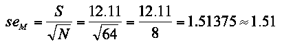
One simple way to look at the mean of a set of scores is to think about it as a sample-based estimate of the mean of the population from which the sample was drawn. Since that estimate is never perfect, it is reasonable to want to know how much error there may be in that estimate of the population mean. The magnitude of this error can be calculated using the seM as follows:
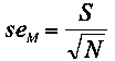
Formula for sem

Where the seM = the standard error of the mean, S = the standard deviation of the scores on a test, and N = the number of examinees who took the test. Consider a test that has a mean of 51, S = 12.11, and N = 64. The seM would be:
Formula for sem to 1.51
This seMis an estimate of the amount of variation due to error that we can expect in sample means. For more information on interpreting the seM, see the discussion below of confidence intervals, limits, and levels.

Standard error of measurement (SEM)
Language testers use reliability estimates to investigate the proportion of consistent variation in scores on a test (for more on this topic see Bachman, 2004; Brown, 1997, 1998, 2002, 2005). Another more useful way to look at the consistency of test scores is to estimate the magnitude of the error by calculating the SEM as follows:
Formula for SEM
Where S = the standard deviation of the scores on a test and rxx' = the reliability estimate for those scores (e.g, Cronbach alpha, K-R20, etc.). Consider a test that has a mean of 31, S of 5.15, and rxx' of .93. The SEM would be:
Formula for SEM = 1.36
This SEM is an estimate of the proportion of variation in the scores that is due to error in the sample score estimates of the examinees' true scores. For more information on interpreting the SEM, see the discussing below of confidence intervals, limits, and levels.

Standard error of estimate (see)
Language testers use regression to predict scores on one test (usually labeled Test Y) from scores on another (usually labeled Test X). One useful way to think about those predictions of Y scores is to estimate how much error there is in the Test Y predictions by calculating the see as follows:
Formula for see
Where Sy = the standard deviation of the scores on Test Y and rxy = the correlation coefficient for the degree of relationship between the Test X scores and those on Test Y. Consider a regression analysis where Sy = 9.54 and rxy = .80. The see would be:
Formula for see = 5.72
This see is an estimate of the amount of variation due to error that we can expect in the predicted Test Y scores based on scores on Test X in a particular regression analysis. For more information on interpreting the see, go to the discussion below of confidence intervals, limits, and levels.

What Are Confidence Intervals, Confidence Limits, Confidence Levels, etc.?

[ p. 24 ]

The confidence intervals, limits, and levels that you asked about in your question, all have to do with the next step after you have the standard error calculated. This next step is to interpret the standard error. In order to do so, we need to understand the differences among confidence intervals, limits, and levels so we can clearly think, talk, and write about our interpretations of standard errors.
Before we turn to using any of the types of standard errors described above to help us interpret our sample statistics, we need to understand that errors are typically assumed to be normally distributed. Since all of the error estimates that we are talking about are standard errors, they are standardized and can be described as shown in Figure 1.
Figure 1
Figure 1. The distribution assumed for standard errors

Notice in Figure 1 that I have provided the percentages that we would expect in each area. For instance, we expect 34.13% of the errors to fall between zero and +1 se. We can also expect about 68% of the errors to fall in the range between -1 se and +1 se (34.13 + 34.13 = 68.26 ≈ 68); similarly, we can expect about 95% of the errors to fall in the range between -2 se and +2 se (13.59 + 34.13 + 34.13 + 13.59 = 95.44 ≈ 95); and we can expect about 99% of the errors to fall in the range between -3 se and +3 se (2.14 + 13.59 + 34.13 + 34.13 + 13.59 + 2.14= 99.72 ≈ 99; note that this last one is rounded to 99% because theoretically we can never account for 100% of error). We use these percents under the distribution to help in establishing confidence intervals.
Coming back to the terminology, a confidence interval is the "range of values of a sample statistic that is likely (at a given level of probability, called a confidence level) to contain a population parameter.2 The interval that will include the population parameter a certain percentage (confidence level) of the time in the long run (over repeated sampling)" (Vogt & Johnson, 2011, p. 67).
In contrast, a confidence level is the degree of confidence, or certainty, that the researcher wants to be able to place in the confidence interval. Put another way, the confidence level is the probability that the parameter being estimated by the statistic falls within the confidence interval. The confidence level is usually expressed as a percentage, but it can also take the form of a proportion (which is also sometimes called a confidence coefficient). The confidence levels cited above were 68%, 95% or 99%. Since the 68% confidence level is only about two-thirds certainty, most researchers in the social sciences select either 95%, which is very confident, or 99%, which is about as confident as we would ever need to be. APA (2010, p. 34) suggests "As a rule, it is best to use a single confidence level, specified on an a priori basis (e.g., a 95% or 99% confidence interval), throughout the manuscript."
And finally, the confidence limits (also known as confidence bounds), are simply the "The upper and lower values of a confidence interval, that is, the values defining the range of a confidence interval" (Vogt & Johnson, 2011, p. 68). So in a case where the ±2 se confidence interval turns out to be 47.98 to 54.02 for the 95% confidence level, the confidence limits are 47.98 and 54.02.
2 About this term parameter, note that statistics are used in samples to estimate analogous parameters in the population from which the sample was drawn. For example, a sample mean statistic, M, is often calculated to estimate the analogous population parameter μ.

[ p. 25 ]

When Are These Statistics Used in Language Testing?

* Why should we care? Consider what the latest APA Manual (APA, 2010) says: "The inclusion of confidence intervals (for estimates of parameters, for functions of parameters such as differences in means, and for effect sizes) can be an extremely effective way of reporting results. Because confidence intervals combine information on location and precision and can often be directly used to infer significance levels, they are, in general, the best reporting strategy. The use of confidence intervals is therefore strongly recommended" (p. 34, italics added).
* In language testing we use confidence intervals to interpret at least the standard error of the mean (seM), standard error of measurement (SEM), and standard error of estimate (see) as I will explain in three separate subsections.

Confidence and the seM
Let's begin by considering the example used above for the seM, where the mean was 51 and the seM turned out to be 1.51. The mean (M) for the sample of 51 is the best estimate that we have of the parameter μ. However, the seM of 1.51 tells us that there is error in that estimate and how big the error is. Since we assume that error is normally distributed, we can estimate the range within which the population mean is likely to exist in probability terms. In this case, we know that the population mean is likely to fall within ±1 seM 68% of the time (34.13 + 34.13 = 68.26 ≈ 68), ±2 seM 95% of the time (34.13 + 34.13 + 13.59 + 13.59 = 95.44 ≈ 95), and ±3 seM 99% of the time (34.13 + 34.13 + 13.59 + 13.59 + 2.14 + 2.14 = 98.58 ≈ 99).
*Hence, we can say that the population μ in our example will fall within plus or minus one confidence interval of the sample mean of 51, that is, from 49.49 to 52.00 about 68% of the time (±1 se in this case = ±1.51; 51 - 1.51 = 49.49; 51 + 1.51 = 52.51). Using the same reasoning, we can say that the population μ in our example will fall within plus or minus two confidence intervals of the sample mean, that is, from 47.98 to 54.02 with 95% probability (±2 se in this case = ±3.02; 51 - 3.02 = 47.98; 51 + 3.02 = 54.02), and that the population μin our example will fall within plus or minus three confidence intervals of the sample mean, that is, from 46.47 to 55.53 with 99% probability (±3 se in this case = ±4.53; 51 - 4.53 = 46.47; 51 + 4.53 = 55.53).

Confidence and the SEM
The SEM calculated in the example above turned out to be 1.36, which can be used to further estimate confidence intervals that indicate how many score points of variation can reasonably be expected with 68%, 95%, or 98% probability around any given point (e.g., a score or a cut-point). Let's say a student scored 32; that student (or any student with that same score) has a 68% probability of getting a score between 30.64 and 33.36 (32 - 1.36 = 30.64; 32 + 1.36 = 33.36) by chance alone if the test were administered repeatedly. Similarly, any examinee with a score of 32 is likely to fall within two SEMs (1.36 + 1.36 = 2.72) plus or minus (32 - 2.72 = 29.28; 32 + 2.72 = 34.72), or a band from 29.28 to 34.72, 95% of the time by chance alone. And finally, an examinee falling within three SEMs (3 x 1.36 = 4.08) plus or minus (32 - 4.08 = 27.92; 32 + 4.08 = 36.08), or a band from 27.92 to 36.08, is likely to fluctuate within that band 99% of the time. In practical terms, language testers most often use the SEM in cut-point decision making, where they may want to at minimum consider gathering additional information about any examinees who have scores within the band of plus or minus one SEM of a given cut-point in order to increase the reliability of that decision making. However, whether the tester chooses a 68%, 95%, or 98% confidence level is a judgment call.
* For additional information on SEM, see Bachman (2004, pp. 171-174), or Brown (2005, pp. 188-190, 193-195).

Confidence and the see

[ p. 26 ]

* The see calculated in the example above turned out to be 5.72, which can be used to further estimate confidence intervals (CIs) that indicate how many score points of variation can reasonably be expected with 68%, 95%, or 98% probability around any given predicted Test Y score in a regression analysis. Test users need to know that the actual Test Y score for any examinee is likely to fall within one see plus or minus of the Test Y score predicted from Test X 68% of the time. Let's say a student's predicted Test Y score is 50; that student (or any student with that same score) has a 68% probability of actually getting a score between 44.28 and 55.72 (50 - 5.72 = 44.28; 50 + 5.72 = 55.72) by chance alone. Similarly, any examinee with a score of 50 is likely to fall within two sees (5.72 + 5.72 = 11.44) plus or minus (50 - 11.44 = 38.56; 50 + 11.44 = 61.44), for a band from 38.56 to 61.44, 95% of the time by chance alone. And finally, an examinee falling within three sees (3 x 5.72 = 17.16) plus or minus (50 - 17.16 = 32.24; 50 + 17.16 = 67.16), or a band from 32.24 to 67.16, is likely to fluctuate within that band 99% of the time. In practical terms, language testers may want to use this information to examine the degree to which the prediction is accurate (e.g., the see of 5.72 in the example here does not seem to indicate a terribly accurate prediction (a glance at the correlation coefficient of .80 above further supports this conclusion), or to make their predictions fairer by at least taking into account the fact that examinees actual scores on Test Y would likely be within the band of plus or minus one see in order to increase the reliability of the prediction making. Whether the tester chooses to use the 68%, 95%, or 98% confidence level is once again judgment call.

Conclusion

In direct answer to the original questions above: I defined confidence intervals, confidence limits, and confidence levels above, and I also explained that we must begin by calculating standard errors of various kinds. I pointed out that we can calculate standard errors for virtually any statistic, but I focused on the seM, SEM, and see because they are the ones that I've often used in my language testing research (note that I have also found myself using standard errors of skewness and kurtosis, standard errors of effect sizes, and others).
* Once we have a standard error value in hand (for whatever statistic), we can then use the confidence intervals, limits, and levels to help us interpret those standard errors. I hope the explanations and examples I have provided here have helped you understand how all of this works and will help you to interpret the standard errors of your own statistics in the future.

References

APA (2010). The publication manual of the American Psychological Association (6th ed.). Washington, DC: American Psychological Association.

Bachman, L. F. (2004). Statistical analyses for language assessment. Cambridge University Press.

Brown, J. D. (1997). Statistics corner: Questions and answers about language testing statistics: Reliability of surveys. Shiken: JALT Testing & Evaluations SIG Newsletter, 1 (2), 18-21. Retrieved from http://jalt.org/test/bro_2.htm

Brown, J. D. (1998). Statistics corner: Questions and answers about language testing statistics: Cloze tests and optimum test length. Shiken: JALT Testing & Evaluations SIG Newsletter, 2 (2), 18-22. Retrieved from http://jalt.org/test/bro_3.htm

Brown, J. D. (1999). Statistics corner: Questions and answers about language testing statistics: Standard error vs. standard error of measurement. Shiken: JALT Testing & Evaluations SIG Newsletter, 3 (1), 20-25. Retrieved from http://jalt.org/test/bro_4.htm

Brown, J. D. (2002). Statistics corner: Questions and answers about language testing statistics: The Cronbach alpha reliability estimate. Shiken: JALT Testing & Evaluations SIG Newsletter, 6 (1), 17-19. Retrieved from http://jalt.org/test/bro_13.htm

Brown, J. D. (2005). Testing in language programs: A comprehensive guide to English language assessment (New edition). New York: McGraw-Hill.

Vogt, W. P., & Johnson, R. B. (2011). Dictionary of statistics & methodology: A nontechnical guide for the social sciences. Thousand Oaks, CA: Sage.


Where to Submit Questions:
Please submit questions for this column to the following e-mail or snail-mail addresses:
browrlj@hawai.edu
JD Brown
Department of ESL, UHM
1890 East-West Road
Honolulu, HI 96822 USA


NEWSLETTER: Topic IndexAuthor IndexTitle IndexDate Index
TEVAL SIG: Main Page Background Links Join

STATISTICS CORNER ARTICLES:
#1   #2   #3   #4   #5   #6   #7   #8   #9   #10   #11   #12   #13   #14   #15   #16  
#17   #18   #19   #20   #21   #22   #23   #24   #25   #26   #27   #28   #29   #30   #31   #32   #33   #34   #35  

last Main Page next
HTML: http://jalt.org/test/bro_35.htm   /   PDF: http://jalt.org/test/PDF/Brown35.pdf

[ p. 27 ]