Shiken:JALT Testing & Evaluation SIG Newsletter
Vol. 8 No. 1. Spring 2004. (p. 22 - 22) [ISSN 1881-5537]
PDF PDF Version

Statistics Corner
Questions and answers about language testing statistics:

Yates correction factor

Photo of JD Brown, c. 2000
James Dean Brown
(University of Hawai'i at Manoa)


* QUESTION: I have a question about Yates' Correction Factor as described in Hatch and Lazaraton (1991, pp. 401-415). The reason I am particularly interested in this is because Mika Shimura of Temple University Japan mentions it in her article on the relationship between personality and advice giving. That article is online at http://jalt.org/pansig/2003/HTML/Shimura.htm. My questions are when do we need to use Yates' Correction Factor and how should it be used?

* ANSWER: Yates' Correction is used with chi-squared analysis under certain conditions. Let me answer your question in the three parts: What is chi-squared analysis? How is Yates' Correction applied? And, when should Yates' Correction be used?

What is Chi-Squared Analysis?

Chi-squared (or X2) analysis is used to compare two or more frequencies to investigate the probability that their values depart from what would be expected by chance alone. Chi-squared is most often used in one-way or two-way X2 analyses. One-way X2 is used to compare the frequencies of different levels of a single variable. So in a study of 100 randomly selected high school students from each of five prefectures in Japan, the frequency of students who went on to university could be studied using chi-squared analysis to see if the frequencies are significantly different from what would be expected by chance alone (for more on chi-squared analysis, see Brown 1988, 2001, or Hatch & Lazaraton, 1991).
I will focus here on two-way X2 analyses, like that in the Shimura example you refer to in your question. Shimura (2003) shows three contingency tables in grey shading (see Example 2), one each for 1st Advice, 2nd Advice, and 3rd Advice. In each contingency table, she compares frequencies in terms of type of advice (with two levels: direct and hedged/indirect) and group (also with two levels: extrovert and introvert). I have reanalyzed her data in Example 1 in order to illustrate how chi-squared analysis would be conducted. The contingency table for 1st Advice is shown in grey in the upper-left portion of Example 1 with the Extrovert, Introvert, and Total labeled on the left hand side and Direct, Hedged/Indirect, and Total labeled across the top.


Example 1: Reanalysis of Shimura's 2004 data
Reanalysis of Shimura's 2004 Data

[ p. 22 ]

Calculating X2 in two-way analyses

The steps for calculating the X2 value in two-way analyses are as follows:

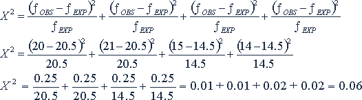
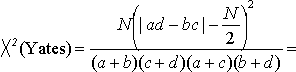
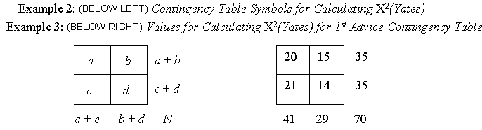
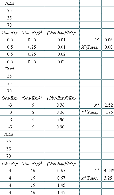
Step 1 - Line up the observed frequencies as shown in the first column just below the 1st Advice contingency table in Example 1.

Step 2 - Calculate the appropriate expected frequency for each observed frequency [multiply the row total for each cell times the column total for the same cell and divide the result by the overall total = (R x C)/T]. For example, the expected frequency for the first cell in the upper left corner of the contingency table in Example 1 (with an observed frequency of 20) would be (R x C)/T = (35 x 41)/70 = 1435/70 = 20.5 for the cell. Example 1 shows the same calculations for each of the four expected frequencies in the 1st Advice contingency table.

Step 3 - For each cell, subtract the expected frequency from the observed frequency, as shown in Example 1 with the observed frequency in the first column minus the expected frequency in the third column giving a result shown in the fourth column. For example, for the first cell, the calculation would be 20 - 20.5 = -0.5.

Step 4 - Square each of the results from Step 3 in the fourth column, and put the result in the fifth column; for the first cell, this results equals 0.25.

Step 5 - Divide each of the squared values obtained in Step 4 by the expected frequency, as shown in the sixth column, which equals 0.25/20.5 = 0.012 or about 0.01 for our example cell.

Step 6 - Repeat steps 2-5 for each cell, as shown for the 1st Advice contingency table.

Step 7 - To get the observed value of X2 for the whole contingency table, add up the Step 5 results for all four cells, which for the 1st Advice contingency table would be 0.01 + 0.01 + 0.02 + 0.02 = 0.06 (the X2 shown for the 1st Advice contingency table, at the right side of Example 1).


[ p. 23 ]

None of these calculations are difficult. In fact, they can easily be done by hand, but the calculations are boring and repetitive so I chose to do them using my spreadsheet program. Using a formula, I would represent the X2 statistic for the two-way analysis in the 1st Advice contingency table as follows:

Calculation of Shimura 2004 Data

Notice that the formula approach is exactly parallel to the approach shown in Example 1. Naturally, if the analysis had a larger number of cells, the formula would have to be expanded to accommodate that larger number of cells. Also notice that X2 values have also been calculated for 2nd Advice and 3rd Advice in Example 1.
Determining the statistical significance of X2. In interpreting such X2 values, we next need to know the probability that such differences between the observed and expected frequencies are due to chance alone. So we investigate the statistical significance of the results. Statistical significance is "the probability that the results of a statistical analysis are due to chance factors" (Brown, 2001, p. 130). For frequency comparisons like those discussed here, statistical significance shows the probability that the differences between observed and expected frequencies are due to chance factors.
Traditionally, the researcher will begin by setting an alpha level, which is the probability level the researcher thinks will be acceptable for deciding if a particular observed difference is or is not due to chance alone. The alpha level is traditionally set at either .01 or .05. Let's set our alpha level at the rather liberal .05 for this Shimura (2003) re-analysis.
Once the alpha level is decided and the X2 observed statistic is calculated, the researcher must turn to a table of critical values of X2 (see, Brown, 1988, p. 192; Brown, 2001, p. 166; or Hatch & Lazaraton, 1991, p. 603). It turns out that the critical value for X2 in such a table for a .05 decision for a 2 x 2 design with 1 degree of freedom [determined by multiplying the number of rows minus one times the number of columns minus one, or (r - 1) x (c - 1) = (2 - 1) x (2 - 1) = 1 x 1 = 1] is 3.842.

[ p. 24 ]

We then compare the observed X2 statistic of 0.06 with the critical X2 value of 3.842 and see that the observed X2 is much lower. We must therefore conclude that this X2 and the associated comparisons are not statistically significant. Looking at the X2 results in Example 1 for the 2nd Advice and 3rd Advice contingency tables, you can see that the resulting observed values of X2 turned out to be 2.52 and 4.24, respectively, and that only the one for the 3rd Advice is significant at p < .05 (i.e., the probability is less than 5% that the comparisons being analyzed occurred by chance alone) as indicated by the asterisk which refers to the p < .05 statement just below the table.

How Should Yates' Correction Be Applied?

For 2 x 2 designs like those in the Shimura (2003) article, Yates' Correction is applied by using a different formula to calculate X2 [I will label this formula X2(Yates)]. The formula adapted slightly from Hatch and Lazaraton (1991) is as follows:

Yates Forumula
Example 2: Contingency Table Symbols for Calculating X<SUP>2</SUP>(Yates) / Example 3: Values for Calculating X<SUP>2</SUP>(Yates) for 1st Advice Contingency Table

To calculate X2(Yates) for the 1st Advice contingency table, I will first substitute all of the appropriate values (shown in Example 3) in the formula and then do the math necessary to find the appropriate value as follows [Note that the | | symbols mean absolute value, so ignore the negative sign in this case]:


[ p. 25 ]

So in this case, X2(Yates) turns out to be 0.00, which is the value recorded in Example 1 for 1st Advice. The values found for 2nd Advice and 3rd Advice are 1.75 and 3.25, respectively. To verify that you have understood the calculation of X2(Yates), try calculating the values for yourself for the 2nd and 3rd Advice contingency tables using the above formula. The significance of these values is determined in the same way shown above for a regular X2 analysis. Using the same critical value of X2 as in the above example (3.842), we find that none of the X2(Yates) values exceed the critical value and so none of them can be considered significant.

When Should Yates' Correction Be Used?

Yates' Correction is typically used in X2 analysis with 1 degree of freedom where expected frequencies of less than 10 are found (some statistics books set that value at 5). A certain amount of controversy surrounds the use of Yates' Correction. Some statisticians argue that expected frequencies lower than five should trigger the use of Yates' Correction, others use 10 as the cut point, and still others argue that Yates' Correction should be used in all 2 x 2 chi-squared analyses.
These issues are touched on in Brown (1988, pp. 190-191) and Hatch and Lazaraton (1991, pp. 404-406), and are discussed in more depth in some of the old tried-and-true nonparametric statistics books (see, for instance, Siegel, 1956; Conover, 1980).

Conclusion

In the Shimura (2003) example, following the thinking of most statisticians, she didn't need to use Yates' correction at all because her smallest expected frequency was 10. Indeed, if she had used the regular chi-squared test, which would have been perfectly rational under these conditions, she would not have had to employ the rather odd strategy of setting her alpha level at .10. Instead, as shown in Example 1, her ordinary chi-squared values for the three analyses (1st Advice, 2nd Advice, and 3rd Advice) would have been .06, 2.52, and 4.24, respectively, the last of which would have been significant at the more traditional p < .05.
Another strategy she could have used (given the controversial nature of Yates' Correction and the pilot nature of her study) would have been to present the results for both the X2 and X2(Yates) statistics and leave the interpretation of those differing results up to the readers.

References

[ p. 27 ]

Brown, J. D. (1988). Understanding research in second language learning: A teacher's guide to statistics and research design. Cambridge: Cambridge University Press.

Brown, J. D. (2001). Using surveys in language programs. Cambridge: Cambridge University Press.

Conover, W. J. (1980). Practical nonparametric statistics (2nd ed.). New York: John Wiley & Sons.

Hatch, E., & Lazaraton, A. (1991). The research manual: Design and statistics for applied linguistics. Boston, MA: Newbury House.

Shimura, M. (2003). Advice giving and personality traits of Japanese university students: A pilot study. In T. Newfields, S. Yamashita, A. Howards, & C. Rinnert (Eds.) Proceedings of the 2003 JALT Pan-SIG Conference. (pp. 28 - 34). . Accessed February 15, 2004 at http://jalt.org/pansig/2003/HTML/Shimura.htm.

Siegel, S. (1956). Nonparametric statistics for the behavioral sciences. New York: McGraw-Hill.


NEWSLETTER: Topic IndexAuthor IndexTitle IndexDate Index
TEVAL SIG: Main Page Background Links Network Join
STATISTICS CORNER ARTICLES:
#1   #2   #3   #4   #5   #6   #7   #8   #9   #10   #11   #12   #13   #14   #15   #16   #17   #18   #19   #20   #21   #22   #23   #24   #25   #26   #27   #28   #29   #30   #31   #32   #33   #34  
last Main Page next
HTML: http://jalt.org/test/bro_19.htm   /   PDF: http://jalt.org/test/PDF/Brown19.pdf

[ p. 27 ]